HUSE: Hierarchical Universal Semantic Embeddings

In this blog post I will go over my PyTorch implementation of HUSE : Hierarchical Universal Semantic Embeddings. This paper is authored by Pradyumna Narayana, Aniket Pednekar, Abishek Krishnamoorthy, Kazoo Sone and Sugato Basu; and can be found here.

Introduction

This paper deals with cross-modal representation learning corresponding to images and text. We want to map images and text to a shared latent space, such that not only embeddings corresponding to a similar class lie closer to each other, but also embeddings which belongs to similar concepts should be close to each other too.

This example is taken from the paper itself. Say we have four classes of instances with us namely: cat, dog, bridge and tower. The embedding space corresponding to these classes can be seen as:

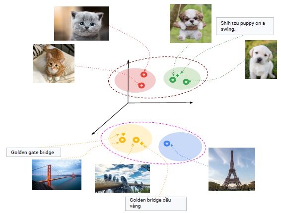
In this space, the embeddings corresponding to a given class (e.g., image and text corresponding to Golden Gate bridge) lie closest to each other. But we can also see that the embeddings corresponding to cat and dog classes are closer to each other as they are semantically similar. Similarly, the embeddings corresponding to bridge and tower are closer to each other.

Implementation details

• Visual: Using the pretrained ResNet50 model to extract embeddings of size 64 from individual images.

• Text: Using BERT embeddings to obtain the text embeddings. For the text associated with each image, we concatenate the embeddings from the last four layers for each token and then average all token embeddings for the text.

• Semantic graph: Constructing an adjacency matrix based on the embeddings extracted from the class names. As class names often contain more than a single word (e.g. bags tote bags tote bags), we use Sentence Transformers that provide sentence level embeddings of class names.

  To build the adjacency matrix, each class name is treated as a vertex and the cosine distance between sentence encoder embeddings of two class names is treated as edge weight.

  This matrix is used to calculate the Graph Loss (which will be defined later.)

Prerequisites

For this implementation, images from the a fashion retail store has been used. The images can be found in ./images folder, and the corresponding .csv files for both training and validation can be found at ./data/ folder at the repo here.

I have also used pre-trained PyTorch models for BERT and Sentence Transformers. Install them from here and here.

Workflow

Let us start by importing basic libraries and defining some variables.

import pandas as pd
import numpy as np
import os
from IPython.display import clear_output

import torch

BATCH_SIZE = 4
EPOCHS = 1

# Chosen arbitrary weights of the three losses
CLASSIFICATION_WEIGHT = 1
GRAPH_WEIGHT = 10
GAP_WEIGHT = 4

device = torch.device("cuda:0" if torch.cuda.is_available()  else 'cpu')

Dealing with data

Let us read the training data and have a look at it.

train_data = pd.read_csv('./data/train_data.csv')
print(train_data.head())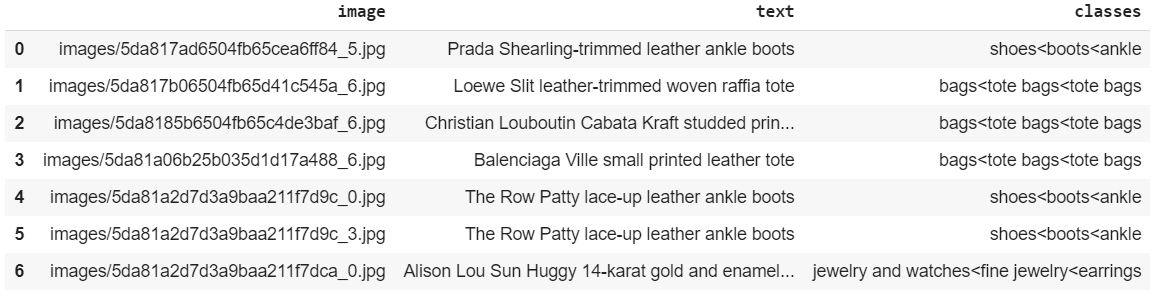

The text associated with each image is the description of the apparel in the picture. If you notice the class for each instance, you will see that it follows a hierarchical pattern, in which each level is seperated by ‘<’.

I’ll show you the unique classes of the training data.

print(train_data.classes.value_counts())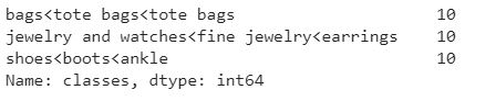

Before proceeding forward, let us clean the data in text column. The clean text will be stores in processed_text column.

import re
def clean_text(x, stopWords):
    x = str(x)
    for punct in "/-'":
        x = x.replace(punct, ' ')
    for punct in '?!.,"#&$%\'()*+-/:;<=>@[\\]^_`{|}~' + '“”’':
        x = x.replace(punct, '')
    x = re.sub('[\d]+', ' ', x) # removes all digit occurences [0-9]
    return x

train_data['processed_text'] = train_data.text.apply(lambda x: "[CLS] " + clean_text(x.lower()) + " [SEP]")
train_data['processed_text'].head(n = 7)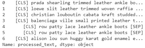

Also for the classes column, I will replace each ‘<’ by whitespace, and store the result in a new column processed_classes

train_data['processed_classes'] = train_data.classes.str.replace('<', ' ')
print(train_data['processed_classes'].head(n = 7))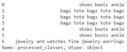

You’ll notice that some classes have repeated words. I will remove the repeated words, but I will maintain the original order of words while doing so.

from collections import Counter, OrderedDict
train_data['processed_classes'] = train_data['processed_classes'].str.split().apply(lambda x: ' '.join(list(OrderedDict.fromkeys(x))))
print(train_data['processed_classes'].head(n = 7))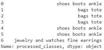

Since Pytorch only takes float values as labels, I also create a feature mapped_class which is just an integer mapping to every class. The classes are mapped to integers using a dictionary classes_dict.

classes = sorted(train_data.processed_classes.unique())
classes_dict = {v:k for (k,v) in enumerate(classes)}
train_data['mapped_classes'] = train_data.processed_classes.map(classes_dict)
train_data['mapped_classes'].head(n = 7)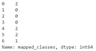

Sentence encoding of the classes

I will use the Sentence Transformer to generate encoding for the classes. From these encodings, I will create an adjacency matrix which will further be used in calculating Graph Loss down the line.

Let us import the required libraries first.

from sentence_transformers import SentenceTransformer
from itertools import combinations
from numpy.linalg import norm
import tqdm

I’ll also import the Sentence Transformer model which will give us BERT embeddings of the each class.

sent_bert = SentenceTransformer('bert-base-nli-mean-tokens')
sent_bert.eval() # Setting the model in evaluation model

I will find the embeddings for each class and store it in sentence_embeddings.

classes = sorted(train_data.processed_classes.unique())
sentence_embeddings = sent_bert.encode(classes)

I will now create an adjaceny matrix which will be used to store cosine distances between class embeddings.

adj_matrix = np.zeros((len(sentence_embeddings), len(sentence_embeddings))) 
print(adj_matrix.shape)

The shape of the adjaceny matrix is 3 x 3, corresponding to the number of classes. I will now store cosine distances between class embeddings in this matrix.

normalised_sentence_embeddings = [i/norm(i) for i in sentence_embeddings]
class_combinations = list(combinations(np.arange(0, len(classes)), r = 2))

for class_tuple in tqdm.tqdm(class_combinations):
    u, v = class_tuple[0], class_tuple[1]
    adj_matrix[class_tuple] = adj_matrix[(v,u)] = 1 - sum(normalised_sentence_embeddings[u] * normalised_sentence_embeddings[v]) 

Datasets and Dataloader

In this section we will define a custom dataset and build our dataloader on top of that.

I’ll import the necessary libraries first.

import math
from PIL import Image
import cv2

import torch
from torch.utils.data.dataset import Dataset
from torchvision import transforms

I will first store the image path and the corresponding text of all instances in array X_train and the targets in y_train.

X_train = train_data.loc[:, ['image', 'processed_text']].values
y_train = train_data['mapped_classes'].values

Now let us create a custom dataset ImageTextDataset which returns the image data, text and target value.

class ImageTextDataset(Dataset):
    def __init__(self, X, y, transforms = None, dir_name = ''): 
      self.filenames = dir_name + X[:, 0]
      self.targets = y
      self.text = X[:, 1]
      self.data_len = len(self.filenames)
      self.transforms = transforms
    
    def __getitem__(self, index):
      filename = self.filenames[index]
      img = Image.open(filename)
      img = self.transforms(img)
      target = self.targets[index]
      text = self.text[index]
      return (img, text, target)

    def __len__(self):
      return self.data_len

Let us also define some transforms for augmenting the image data.

transform = transforms.Compose([transforms.RandomRotation(5),
                        transforms.RandomResizedCrop(284, scale = (0.9, 1.0)),
                        transforms.ColorJitter(brightness=0.2, contrast=0.1, hue=0.07), # Adding some random jitter
                        transforms.ToTensor(),
                        transforms.Normalize((0.485, 0.456, 0.406), (0.229, 0.224, 0.225)) # ImageNet stats
                        ])

Creating a train dataloader based on our ImageTextDataset.

trainset = ImageTextDataset(X_train, y_train, transform)
trainloader = torch.utils.data.DataLoader(trainset, shuffle = True, batch_size = BATCH_SIZE, drop_last = True)

What does our train dataloader return?

trainiter = iter(trainloader)
images, texts, targets = next(trainiter)

images is nothing but a tensor of size [B, 3, 284, 284], where B = BATCH_SIZE and 284 is the size we had mentioned in the transforms.

print('Size of images tensor:', images.shape)

What about texts? It is tuple of length = BATCH_SIZE, and each element is the processed text of the given instance

for text in texts:
  print(text)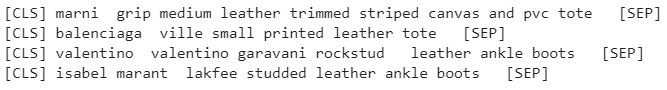

And targets? It is tensor of size = BATCH_SIZE having the ground truth labels of the instances.

print(targets)

Towers model

In this section I will define our model Towers. This model takes the image and text embeddings as input, and passes each embedding through a number of MLP layers. In the end, the image and text embeddings and passed through a shared layer.

I have decided to make a single model for both image and text towers.

import torch.nn as nn

class Towers(nn.Module):
  
  def __init__(self, num_classes = 3, image_weight = 0.5, text_weight = 0.5):
    super(Towers, self).__init__()

    img_layers = self.LinearBlock(64, 512) + sum([self.LinearBlock(512, 512) for i in range(4)], [])
    text_layers = self.LinearBlock(3072, 512) + self.LinearBlock(512, 512)

    # The output of the second last layer of ResNet50 is a 2048 featured vector 
    self.downsize = nn.Sequential(*self.LinearBlock(2048, 64, 0.0)) 
    
    # unpacking the img_layers list  --> Sequential of 5 linear_blocks
    self.img_features = nn.Sequential(*img_layers)
    # unpacking the text_layers list  --> Sequential of 2 linear_blocks
    self.text_features = nn.Sequential(*text_layers) 

    self.shared = nn.Linear(512, num_classes)
    self.batchnorm = nn.BatchNorm1d(512)

    self.image_weight = image_weight
    self.text_weight = text_weight
      
  def LinearBlock(self, in_features, out_features, dropout_p = 0.15):
    block = [nn.Linear(in_features, out_features), nn.BatchNorm1d(out_features), nn.LeakyReLU(0.1), nn.Dropout(dropout_p)]
    return block

  def forward(self, img_embedding, text_embedding): #  takes the image and text embedding as input
    
    img_f = self.img_features(self.downsize(img_embedding)) # finds image features
    text_f = self.text_features(text_embedding) # finds text features

    # L2 normalisation of image features
    img_f_norm = torch.norm(img_f, p=2, dim=1).detach() 
    img_f = img_f.div(img_f_norm.unsqueeze(1))

    # L2 normalisation of text features
    text_f_norm = torch.norm(text_f, p=2, dim=1).detach()
    text_f = text_f.div(text_f_norm.unsqueeze(1))

    image_shared_output = self.shared(img_f)
    text_shared_output = self.shared(text_f)
    shared_output = (image_shared_output * self.image_weight) + (text_shared_output * self.text_weight)

    return shared_output, image_shared_output, text_shared_output

Note that the Towers model returns 3 outputs. The weighted embedding of image and text features after passing through the shared layer, as well as image and text embeddings individually after passing through the shared layer.

Utility functions

Before defining the custom loss functions, I will define some utility functions that help this implementation run smoothly.

First, I will define a function get_encoding that will generate the Bert embeddings of the text data that we get from our training dataloader. I have left the comments alongside the code for better understanding.

from pytorch_pretrained_bert import BertTokenizer, BertModel, BertForMaskedLM
tokenizer = BertTokenizer.from_pretrained('bert-base-uncased')

def get_encoding(text):
    tokenized_text = tokenizer.tokenize(text) # It expects that the string starts with [CLS] and ends with [SEP] tags.
    indexed_tokens = tokenizer.convert_tokens_to_ids(tokenized_text) # Converting tokens to ids in the BERT vocab
    segments_ids = [1] * len(tokenized_text)

    tokens_tensor = torch.tensor([indexed_tokens]).to(device)
    segments_tensors = torch.tensor([segments_ids]).to(device)

    with torch.no_grad():
      encoded_layers, _ = bert(tokens_tensor, segments_tensors)

    token_embeddings = torch.stack(encoded_layers, dim=0).squeeze(1) 
    token_embeddings = token_embeddings.permute(1,0,2) # Correcting the dimensions

    # Getting the embeddings only from the last 4 layers
    token_vecs_cat = []
    for token in token_embeddings:
        cat_vec = torch.cat((token[-1], token[-2], token[-3], token[-4]), dim=0) 
        token_vecs_cat.append(cat_vec)
    
    return torch.mean(torch.stack(token_vecs_cat, dim = 0), dim = 0) # returning the mean of the last 4 layer embeddings 

I now define a function graph_loss_utility whose output will be used by our graph loss function to compute the loss. It takes in input, the predicted classes outputs, the ground truth targets and adjacency matrix of class embeddings as input.

what does this graph_loss_utility function do?

1. First for a given batch, I find the total combinations of 2 tuples (from 0 to B - 1) that can be made. Note that I do not include tuples like (1,1), (2,2), (0,0) etc because they do not contribute to the loss. I store these combinations in a list x_tuples.

2. For each tuple in x_tuples, I find the real target value of each x in that tuple and store them as a tuple. Hence creating the list of tuples target_tuples. Since we only have 3 classes in this data, the targets will be 0, 1 or 2.

3. For each tuple in target_tuples, we find the cosine distance between the two targets in the tuple using the adjacency matrix that we had created earlier. Hence creating a list A_ij.

4. We have got with us an output tensor of size (B, 3), where 3 = # classes and B = BATCH_SIZE. For each tuple in x_tuples, I find the cosine distance between the two examples in that tuple.

   e.g. (0,1) be the tuple in x_tuples, then I will find the distance between output[0] and output[1].

This function finally returns A_ij and cosine_x, both filtered by the margin parameter. See the original paper for more details on this topic.

import torch.nn.functional as F

def graph_loss_utility(outputs, targets, adj_matrix, margin = 0.2):

  x_tuples = list(combinations(range(outputs.shape[0]), r = 2)) # [(0, 1), (0, 2), (0, 3), (1, 2), (1, 3), (2, 3)] 
                                                                # for the given batch_size = 4 --> 4C2 = 6, hence 6 tuples
  target_tuples = [tuple(targets[[*tuple_]].detach().cpu().numpy()) for tuple_ in x_tuples] # [(1, 2), (1, 0), (1, 2), 
                                                                                           # (2, 0), (2, 2), (0, 2)] --> 6 tuples here too.

  # Using target_tuples, we find the cosine distance values between these classes using the adjacency matrix -- > A_ij
  A_ij = torch.tensor([adj_matrix[tuple_] for tuple_ in target_tuples]).to(device)
  
  # Using x_tuples and outputs, we find the cosine distance between two points in each tuple corresponding to real target index
  cosine_x = torch.stack([F.cosine_similarity(outputs[tuple_[0]], outputs[tuple_[1]], dim = 0, ) for tuple_ in x_tuples])

  sigma_x = torch.tensor([1 if ((A_ij[i] < margin) and (cosine_x[i] < margin)) else 0 for i in range(len(A_ij)) ]).to(device)
  
  return (A_ij * sigma_x).float(), cosine_x * sigma_x

Loss functions

The authors have employed three losses in the paper namely:

• Classification Loss - It is essentially a Cross Entropy loss between the outputs of our model and the real targets

 cl_loss_type = nn.CrossEntropyLoss()

 def classification_loss_fn(outputs, targets):
  return cl_loss_type(outputs, targets)
 

• GAP Loss - This loss enforces that both image and text embeddings of a single instance should be as similar as possible.

def gap_loss_fn(image_features, text_features): 
  return torch.mean(1 - F.cosine_similarity(image_features, text_features))

• Graph Loss - is essentially a slightly modified MSE Loss function and it make our embeddings semantically meaningful.

gr_loss_type = nn.MSELoss()

def graph_loss_fn(outputs, targets, adj_matrix): 
  g1, g2 = graph_loss_utility(outputs, targets, adj_matrix)
  return gr_loss_type(g2, g1)/len(g1)

Explaining the graph loss function

How will our graph_loss_fn make embeddings semantically meaningful?

For any x-tuple pair, say (0,1) having real target tuple, say (1, 2), we find the squared difference between

• Cosine distance of embeddings of outputs[0] and outputs[1].
• Cosine distance of class embeddings of targets 1 and 2 (can be found easily from the adjacency matrix).

This is done for all the tuples, and a MSE like loss function is generated from these. Each squared error term can be minimised if the cosine distance of embeddings is as close as possible to the value obtained from the adjacency matrix.

If say the value from the matrix is low (meaning that class similarity is high), this forces the cosine distance of the input embeddings to be low too. In contrast, if the value from the matrix is high (meaning that class similarity is low), this forces the cosine distance of the input embeddings to be high as well.

This type of regularisation enforces semantically similar classes to be closer to each other, and dis-similar classes to be farther away.

Training our model!

Finally we have arrived at the stage when we can train our model!

Let us begin by importing the necessary modules.

import torchvision.models as models

# Importing pre-trained resnet50 and removing the last dense layer to generate image embeddings
resnet50 = models.resnet50(pretrained = True)
resnet50 = torch.nn.Sequential(*(list(resnet50.children())[:-1])).to(device).eval() 
# Importing pre-trained bert model for generating text embeddings
bert = BertModel.from_pretrained('bert-base-uncased').to(device).eval()

for param in resnet50.parameters():
    param.requires_grad = False

for param in bert.parameters():
    param.requires_grad = False

I am defining train function for training a single epoch.

def train(epoch, model, opt, classification_loss_fn, graph_loss_fn, gap_loss_fn, 
          classification_weight, graph_weight, gap_weight, batch_size, 
          log_interval = 50, device = device):
  
  loss_agg =  0
  classification_loss_agg = 0
  graph_loss_agg = 0
  gap_loss_agg = 0

  trainloader = torch.utils.data.DataLoader(trainset, shuffle = True, batch_size = batch_size, drop_last= True)

  for batch_id, data in tqdm.tqdm(enumerate(trainloader)):

    imgs, texts, targets = data
    imgs = imgs.to(device)
    targets = targets.to(device)

    img_embeddings = resnet50(imgs).to(device).squeeze(2).squeeze(2)
    text_embeddings = torch.stack([get_encoding(text) for text in texts]).to(device)
    
    opt.zero_grad()
    outputs, imgs_f, texts_f = model(img_embeddings, text_embeddings)

    classification_loss = classification_loss_fn(outputs, targets)
    graph_loss = graph_loss_fn(outputs, targets, adj_matrix) 
    gap_loss = gap_loss_fn(imgs_f, texts_f)
    loss= (classification_loss * classification_weight) + (graph_loss * graph_weight) + (gap_loss * gap_weight)
    
    loss_agg += loss.item()
    classification_loss_agg += classification_loss.item()
    graph_loss_agg += graph_loss.item()
    gap_loss_agg += gap_loss.item()
    
    loss.backward()
    opt.step()

    if (batch_id + 1) % log_interval == 0:
      mesg = "\tEpoch {}:  [{}/{}]\tloss: {:.6f}\tclf_avg_loss: {:.6f}\tgraph_avg_loss: {:.6f}\tgap_av_loss: {:.6f}\tloss_avg: {:.6f}".format(
                        epoch + 1, batch_size * (batch_id + 1), len(trainset), loss.item(),
                        classification_loss_agg/(batch_id + 1), graph_loss_agg/(batch_id + 1), gap_loss_agg/(batch_id + 1), loss_agg/(batch_id + 1))
      print(mesg)

Let us define the train_setup function also, which handles the complete training of our model. I have also added the ability to checkpoint the model after every epoch (if checkpoints directory has been given). After the training is complete, you can also save the model (if model save directory is given).

def train_setup(model, classification_loss_fn, graph_loss_fn, gap_loss_fn, opt, epochs, 
                classification_weight = CLASSIFICATION_WEIGHT, graph_weight = GRAPH_WEIGHT, gap_weight = GAP_WEIGHT,
                batch_size = BATCH_SIZE, log_interval = 50,
                checkpoint_dir = None, save_model_dir = None, device = device):
  
  model = model.to(device)
  model.train()

  for e in range(epochs):
    train(e, model, opt, classification_loss_fn, graph_loss_fn, gap_loss_fn, classification_weight, graph_weight, gap_weight, batch_size, device = device)

    # Checkpointing model after every epoch
    if checkpoint_dir is not None and os.path.exists(checkpoint_dir):
      model.eval().cpu()
      ckpt_model_path = os.path.join(checkpoint_dir, 'checkpoint.pth.tar')
      torch.save({'epoch': e + 1, 'network_state_dict': model.state_dict(),
                  'optimizer' : opt.state_dict()}, ckpt_model_path)
      model.to(device).train()
  
  #Saving the model after the training is complete
  if save_model_dir is not None and os.path.exists(save_model_dir):
    model.eval().cpu()
    save_model_filename = "epoch_" + str(epochs) + "_" + str(batch_size) + ".pth.tar"
    save_model_path = os.path.join(save_model_dir, save_model_filename)
    torch.save(model.state_dict(), save_model_path)
    print("\nDone, trained model saved at", save_model_path)

Let us train our model for one epoch:

from torch.optim import Adam, RMSprop, AdamW
model = Towers(len(classes))

opt = RMSprop(model.parameters(),lr = 1.6192e-05, momentum = 0.9) # used the same optimiser and lr of the paper

epochs = EPOCHS
batch_size = BATCH_SIZE
log_interval = 50

train_setup(model = model, classification_loss_fn = classification_loss_fn, graph_loss_fn = graph_loss_fn, 
            gap_loss_fn = gap_loss_fn, opt = opt, epochs = epochs, 
            classification_weight = CLASSIFICATION_WEIGHT, graph_weight = GRAPH_WEIGHT, gap_weight = GAP_WEIGHT,
            batch_size = batch_size, log_interval = log_interval, device = device)

The data that I have provided in the repo consists of only 31 examples belonging to 3 classes. However I trained the model on 1,22,164 instances having 48 classes for one epoch.

50it [02:31,  2.97s/it]	Epoch 1:  [200/30541]	loss: 7.744383	clf_avg_loss: 3.657022	graph_avg_loss: 0.096067	gap_av_loss: 0.744851	loss_avg: 7.597097
100it [04:59,  3.07s/it]	Epoch 1:  [400/30541]	loss: 6.726626	clf_avg_loss: 3.469530	graph_avg_loss: 0.100957	gap_av_loss: 0.740253	loss_avg: 7.440107
150it [07:29,  3.00s/it]	Epoch 1:  [600/30541]	loss: 6.496047	clf_avg_loss: 3.333538	graph_avg_loss: 0.099195	gap_av_loss: 0.737363	loss_avg: 7.274938
200it [10:00,  3.15s/it]	Epoch 1:  [800/30541]	loss: 6.373997	clf_avg_loss: 3.189371	graph_avg_loss: 0.099426	gap_av_loss: 0.734746	loss_avg: 7.122612
250it [12:36,  2.86s/it]	Epoch 1:  [1000/30541]	loss: 6.358969	clf_avg_loss: 3.123342	graph_avg_loss: 0.100168	gap_av_loss: 0.733780	loss_avg: 7.060136
300it [15:03,  2.95s/it]	Epoch 1:  [1200/30541]	loss: 6.889596	clf_avg_loss: 3.066376	graph_avg_loss: 0.100879	gap_av_loss: 0.731601	loss_avg: 7.001565
                                                                            .
                                                                            .
                                                                            .
                                                                            .
7450it [6:06:50,  3.15s/it]	Epoch 1:  [29800/30541]	loss: 2.219154	clf_avg_loss: 1.434936	graph_avg_loss: 0.027754	gap_av_loss: 0.561705	loss_avg: 3.959295
7500it [6:09:28,  3.27s/it]	Epoch 1:  [30000/30541]	loss: 3.319882	clf_avg_loss: 1.431660	graph_avg_loss: 0.027609	gap_av_loss: 0.561327	loss_avg: 3.953057
7550it [6:12:01,  3.22s/it]	Epoch 1:  [30200/30541]	loss: 2.759284	clf_avg_loss: 1.429620	graph_avg_loss: 0.027476	gap_av_loss: 0.560845	loss_avg: 3.947764
7600it [6:14:33,  3.11s/it]	Epoch 1:  [30400/30541]	loss: 3.492151	clf_avg_loss: 1.426620	graph_avg_loss: 0.027340	gap_av_loss: 0.560462	loss_avg: 3.941868

The Average Loss over the epoch reduced from 7.440107 in the first batch iteration to 3.941868 in the last one.

Same decreasing trend in average loss can be seen for individual loss components :

1) Average Classification Loss : 3.469530 to 1.426620

2) Average Graph Loss : 0.100957 to 0.027340

3) Average GAP Loss: 0.740253 to 0.560462

Evaluating our model

Once the training is complete, we can test our model on the validation data. The validation data can be found at ./data/eval_data.csv in the repo.

Let us read the validation data first.

eval_data = pd.read_csv('eval_data.csv')
print(eval_data.head())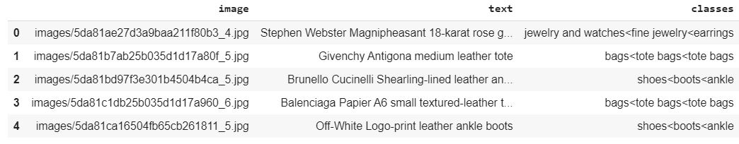

I’ll also clean the text and do other processing as I did during the training phase.

eval_data['processed_text'] = eval_data.text.apply(lambda x: "[CLS] " + clean_text(x.lower()) + " [SEP]")

eval_data['processed_classes'] = eval_data.classes.str.replace('<', ' ')
eval_data['processed_classes'] = eval_data['processed_classes'].str.split().apply(lambda x: ' '.join(list(OrderedDict.fromkeys(x))))

eval_data['mapped_classes'] = eval_data.processed_classes.map(classes_dict)
print(eval_data.loc[:, ['image', 'processed_text', 'processed_classes', 'mapped_classes']].head(n = 7))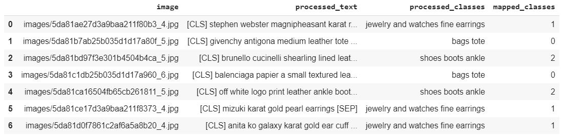

I will first store the image path and the corresponding text of all validation instances in array X_val and the targets in y_val.

X_val = eval_data.loc[:, ['image', 'processed_text']].values
y_val = eval_data['mapped_classes'].values

Now I will create a validation dataloader based on ImageTextDataset.

transform = transforms.Compose([transforms.ToTensor(),
                               transforms.Normalize((0.485, 0.456, 0.406), (0.229, 0.224, 0.225))])
valset = ImageTextDataset(X_val, y_val, transform)
valloader = torch.utils.data.DataLoader(valset, shuffle = True, batch_size = 1)
print(len(valloader))

Let us also define the validation function val which will evalute the model for us.

def val(classification_loss_fn, graph_loss_fn, gap_loss_fn):
  model.eval() # Keep the Towers model in evaluation mode
  val_loss = 0
  correct = 0
  confusion_matrix = np.zeros([len(classes), len(classes)])
  
  valloader = torch.utils.data.DataLoader(valset, shuffle = True, batch_size = 1)

  resnet50 = models.resnet50(pretrained = True)
  resnet50 = torch.nn.Sequential(*(list(resnet50.children())[:-1])).to(device).eval() 
  bert = BertModel.from_pretrained('bert-base-uncased').to(device).eval()

  for param in resnet50.parameters():
      param.requires_grad = False

  for param in bert.parameters():
      param.requires_grad = False
  
  with torch.no_grad():
    for data in valloader:
      
      img, text, target = data
      img = img.to(device)
      target = target.to(device)

      img_embeddings = resnet50(img).to(device).squeeze(2).squeeze(2)
      text_embeddings = torch.stack([get_encoding(text) for text in text]).to(device)
      
      pred, img_f, text_f = model(img_embeddings, text_embeddings)
      
      cl_loss = classification_loss_fn(pred, target)
      gr_loss = graph_loss_fn(pred, target, adj_matrix) 
      gap_loss = gap_loss_fn(img_f, text_f)

      loss= cl_loss + gr_loss + gap_loss
      val_loss += loss.item()
      
      pred = pred.data.max(1)[1]
      correct += pred.eq(target.data).sum().item()
      for x, y in zip(pred.cpu().numpy(), target.cpu().numpy()):
        confusion_matrix[x][y] += 1
      
    val_loss /= len(valloader.dataset)
    val_accuracy = 100.0 * correct / len(valloader.dataset)

    return val_loss, val_accuracy, confusion_matrix

This function will return the validation loss, validation accuracy, and the confusion matrix for our prediction.

val_loss, val_accuracy, confusion_matrix = val(classification_loss_fn, graph_loss_fn, gap_loss_fn)

Conclusion

Did a PyTorch implementation of HUSE, to learn a universal embedding space that incorporates semantic information. The model learns a new universal embedding space that still has the same semantic distance as the class label embedding space.